(Image source)

We all know what a curve is. Here are some examples.

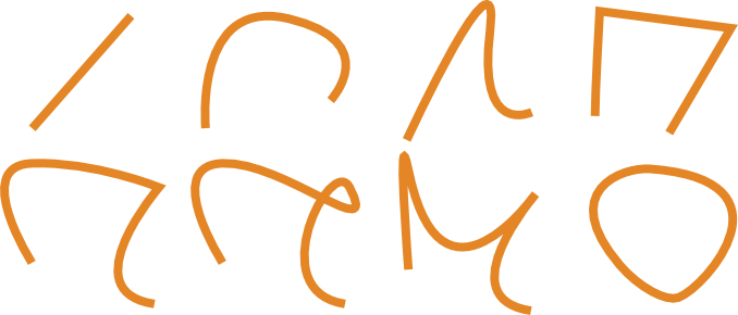
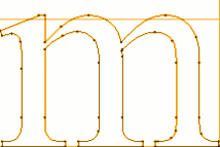
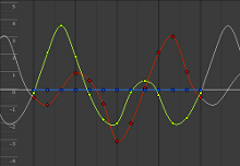
A Bézier curve is a type of curve that is easy to use, and can describe many shapes. Bézier curves are famously used for representing characters in fonts, and shapes in vehicle design. Bézier curves are also used in vector art packages for curve drawing, and in 3D animation tools to represent animation paths.

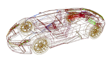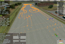
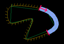
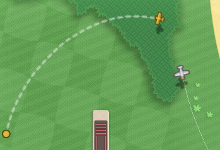
In games, Bézier curves are sometimes useful to describe paths: the racing line in a racing game, or the line in line-drawing games such as Flight Control, or the looping butterfly that enlivens an RPG.

Bézier curves are popular because their mathematical descriptions are compact, intuitive, and elegant. They are easy to compute, easy to use in higher dimensions (3D and up), and can be stitched together to represent any shape you can imagine.

In this guide, I give you the instructions necessary to implement algorithms for using Bézier curves in your games.

Mathematical Description

Let’s start with the mathematics. Mathematically, we describe a Bézier curve by a function. The function takes a parameter \(t\). The value of the function is a point on the curve; it depends on the parameter \(t\), and on a set of points, called the control points. The first and last control points are the endpoints of the curve. Generally, the curve does not pass through the other control points.

The value \(t\) can range from 0 to 1. The value 0 corresponds to the start point of the curve; the value 1 corresponds to the endpoint of the curve. Values in between correspond to other points on the curve.

Here is an example of the simplest type of Bézier curve, a line-segment:

$$[x, y] = (1 – t)P_0 + tP_1$$

This is shorthand notation for the two equations that give the coordinates separately (see Vector Fundamentals):

$$x = (1 – t)P_{0x} + tP_{1x}$$

$$y = (1 – t)P_{0y} + tP_{1y}$$

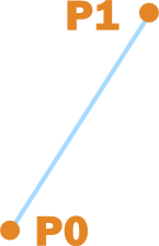
The points \(P_0\) and \(P_1\) are the control points. When \(t = 0\), the right hand side equals the first control point – the start of the line segment. When \(t = 1\), we get the point \(P_1\), the second control point and the end of the line segment.

For more interesting shapes, we need more control points. The number of control points determines the degree of the curve. Two control points are necessary for a linear (degree-one) curve, such as the line-segment above. For degree-two, or quadratic curves, we need three control points.

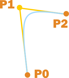
Here is the formula:

$$[x, y] = (1 – t)^2P_0 + 2(1 – t)tP_1 + t^2P_2$$

Cubic curves (or degree-three curves) are the most frequently used, and so we will discuss cubic curves in this guide. They require four control points, and chances are you are already quite familiar with using them in vector drawing packages (yes, those handles used to change the shape of curves in Freehand or Inkscape are really control points).

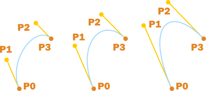
The yellow lines are in the same direction as the tangents at the endpoints. The longer these yellow segments, the stronger the “pull” towards the tangent.

The formula for cubic Bézier curves is:

$$[x, y] = (1 – t)^3P_0 + 3(1 – t)^2tP_1 + 3(1 – t)t^2P_2 + t^3P_3$$

You will rarely need higher degree curves. If you do, the formula is simple, but requires some knowledge of binomial coefficients. You can find the detail in one of the sources at the end of the article.

Cases

In geometry, there are always more cases than you first think of, which can lead to subtle and difficult-to-find bugs.

These are all valid 2D Bézier curves:

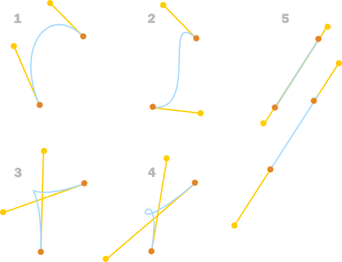
All endpoints are the same distance apart. 1. Curve without inflection, cusp or loop. 2. Curve with inflection and no cusp or loop. 3. Curve with cusp. 4. Curve with loop. 5. Straight line. (An inflection point is a point where the curve changes it bending direction.)

The degenerate case 5 is the most complex. The following sub-cases are possible:

• no overlap
• curve overlaps double at one or both endpoints
• curve overlaps triple somewhere between the endpoints

There is a 6th case that occurs when all four control points coincide: the resulting curve is a single point. Note that the curve does not degenerate to a point when only the end-points coincide: all four control points must coincide. For a technical treatment of this topic, see A Geometric Characterization of Parametric Cubic Curves (1.6 MB PDF) by Stone and De Rose. The article Inflection points of a cubic Bezier explains how to calculate points of inflection, and provides interactive Java applets to illustrate the concepts.

In 3D, loops and overlaps are less of a problem, since they only occur when all the points lie in the same plane – exactly when the curve is 2D. It is still possible for the curve to change direction in 3D (as it does in cases 2, 4, and 5).

When implementing Bézier curve algorithms, carefully consider whether these cases can occur, and whether the algorithm handles them correctly. Be especially wary of coincident control points – trying to normalize the zero vector that might crop up in calculations can lead to a nasty crash.

Implementation

It is straightforward to translate the mathematical formula to code. In the implementation below, we optimised the algorithm somewhat by storing and reusing partial results.

The code is in C#, but should be trivial to translate to Java, C++ and most other languages.

(The following functions all work for 2D if Vector3 is replaced by Vector2.)

Vector3 CalculateBezierPoint(float t,
  Vector3 p0, Vector3 p1, Vector3 p2, Vector3 p3)
{
  float u = 1 – t;
  float tt = t*t;
  float uu = u*u;
  float uuu = uu * u;
  float ttt = tt * t;
 
  Vector3 p = uuu * p0; //first term
  p += 3 * uu * t * p1; //second term
  p += 3 * u * tt * p2; //third term
  p += ttt * p3; //fourth term
 
  return p;
}

Drawing Bézier Curves

Now that we have a way to calculate points on the Bézier curve, we need a way to draw the curve.

For images, the simplest approach is to use small increments of t to calculate successive points:

for(int i = 0; i <= SEGMENT_COUNT; i++)
{
  t = i / (float) SEGMENT_COUNT;
  Vector3 pixel = CalculateBezierPoint(t, p0, p1, p2, p3);
  DrawPixel(pixel); //assume this function can handle Vector3
}

This approach suffers from these problems:

• it is hard to know what value to use for the increment;
• pixels might be overdrawn;
• pixels might be missed.

More sophisticated algorithms use an adaptive increment (of t) to overcome these problems. Anti-aliasing the curve will even give better results, making the curve appear very smooth and crisp. A good source for drawing curves (and a load of other useful topics) is Computer Graphics and Computer Modelling by David Salomon.

A simpler alternative is to draw lines instead of pixels. This method is also more appropriate for drawing curves using graphics hardware.

q0 = CalculateBezierPoint(0, p0, p1, p2, p3);
 
for(int i = 1; i <= SEGMENT_COUNT; i++)
{
  t = i / (float) SEGMENT_COUNT;
  q1 = CalculateBezierPoint(t, p0, p1, p2, p3);
  DrawLine(q0, q1);
  q0 = q1;
}

Because we need not worry about skipping pixels, we can choose a larger increment and reduce overdrawing. But it is still hard to choose the increment properly.

Another algorithm uses recursive subdivision. It generally gives fewer drawing points for the same level of accuracy than the previous algorithm. However, it does not handle all curves with inflections or loops correctly, and should not be used when such curves can occur.

Here is the algorithm:

1. Start at the endpoints: the curve points at \(t = 0\) and \(t = 1\).
2. Calculate the halfway point (at \(t = 0.5\), the first time round).
3. If the angle between formed by the two line segments is smaller than a threshold value, then add the point as a drawing point. Now recursively repeat with each half of the curve. Stop the algorithm when no more division is possible, or the line segments reach a minimal length.

The figure below shows a worked example.

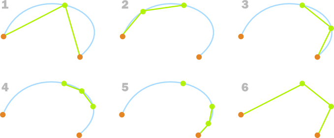
1. We start with the two endpoints and the point in between. We check the angle formed between the two line segments. It is too small, so we add the point in between as a drawing point. 2. We then do the same for the left part of the curve. In this case, the angle is large enough, so we do not add the point, and we do not subdivide further. 3. We do the same for the right part of the curve. In this case, the angle is too small, so we add the new point as a drawing point, and subdivide. 4. and 5. We do the same for the two halves of the previous step. In each case, the angle is large enough, so the new points are not added, and no subdivision is necessary. 6. The final set of points used to draw the curve.

Below is the recursive algorithm in code. The tricky part is inserting drawing points at the right place in the list so that they remain in the right order. We check the dot product of normalised segments, instead of checking the angle directly (see Vector Recipes for an explanation of this trick). This check uses a > in the inequality, instead of the < that we would use if we had checked the angles directly.

float FindDrawingPoints(float t0, float t1, int insertionIndex,
  List pointList)
  //returns the number of points added.
{
  tMid = (t0 + t1) / 2;
  p0 = bezierCurve(t0);
  p1 = bezierCurve(t1);
 
  if(p0 – p1.sqrMagnitude < MINIMUM_SQR_DISTANCE)
  {
    return 0;
  }
 
  pMid = bezierCurve(tMid);
  leftDirection = (p0 – pMid).Normalised;
  rightDirection = (p1 – mMid).Normalised;
 
  if(Dot(leftDirection, rightDirection) > threshold)
  {
    int pointsAddedCount = 0;
 
    pointsAdded +=
      FindDrawingPoints(t0, tMid, insertionIndex,  pointList) 
 
    pointList.insert(insertionIndex + pointsAdded, pMid);
    pointsAdded++;
 
    pointsAdded +=
      FindDrawingPoints(tMid, t1, insertionIndex + pointsAdded, pointList);
    return pointsAdded;
  }
  return 0;
}

The following function makes the base call to the recursive function:

void FindPoints()
{
  List pointList = new List();
  p0 = bezierCurve(0);
  p1 = bezierCurve(1);
  pointList.Add(p0);
  pointList.Add(p1);
 
  int pointsAdded = FindPoints(0, 1, 1, pointList);
 
  assert(pointsAdded + 2 == pointsList.Count);//sanity check
}

A few notes:

• The minimum distance check is necessary to prevent problems with normalizing very short vectors. It also prevents unnecessary calculations.
• The threshold value is surprisingly close to -1. A good value to start with is -0.99.
• The algorithm does not work well for curves that contain infections or loops. Below is an example of what can happen when we apply it to a curve with an inflection.

An example where the algorithm will give a poor result. In this case, the angle is larger than the threshold, so no subdivision will occur. The resulting line segment is a poor representation of the curve.

Stitching curves together: Bézier paths

When we want to represent a complicated curve, we have two options:

• use a single Bézier curve with a high degree;
• split the curve into smaller segments, and use a lower degree Bézier curves for each segment.

The last type of curve is called a Bézier path. Bézier paths are usually simpler and more efficient to use than higher degree curves, and is the method described here. (Many sources use the word Bézier curve to also refer to what we call Bézier paths, relying on context to make it obvious which is meant. When implementing these curves however, the distinct terms help us give better variable names).

The implementation described here is just one of many possibilities. We define a class, which creates a list of the control points of the Bézier curves which themselves make up a Bézier path. Because the segments are connected end-to-end, the last and first control points of successive curves are the same, and we can omit one of the duplicates. The illustration shows an example of a Bézier path made out of four Bézier curves. In this case, the list contains 13 points, as shown on the left.

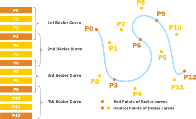
If we decide to draw the curve with line segments, it is convenient to cache the endpoints of the line segments, and update them whenever the curve changes. The following algorithm calculates all the drawing points (endpoints of line segments).

class BezierPath
{
  List controlPoints;
 
  Vector3 CalculateBezierPoint(float t,
  Vector3 p0, Vector3 p1, Vector3 p2, Vector3 p3){...}
 
  List GetDrawingPoints()
  {
    List drawingPoints = new List();
    for(int i = 0; i < controlPoints.Count - 3; i+=3)
    {
      Vector3 p0 = controlPoints[i];
      Vector3 p1 = controlPoints[i + 1];
      Vector3 p2 = controlPoints[i + 2];
      Vector3 p3 = controlPoints[i + 3];    
 
      if(i == 0) //Only do this for the first endpoint.
                 //When i != 0, this coincides with the end
                 //point of the previous segment
      {
        drawingPoints.Add(CalculateBezierPoint(0, p0, p1, p2, p3));
      }    
 
      for(int j = 1; j <= SEGMENTS_PER_CURVE; j++)
      {
        float t = j / (float) SEGMENTS_PER_CURVE;
        drawingPoints.Add(CalculateBezierPoint(t, p0, p1, p2, p3));
      }
    }
 
    return drawingPoints;
  }
}

It is easy to use the recursive algorithm to get the points instead. An example can be found in the downloadable code at the end of this article.

Final Advice

When implementing Bézier paths, you can make your life a lot easier by doing the following:

• Enable debug modes for drawing control points, Bézier endpoints, drawing points, and tangents.
• Print out the number of drawing points and control points: this makes it easier to see whether your algorithms produce a sane number of points.

Finally, Bézier curves are great, but don’t use them when a collection of short, straight line-segments will do.

• Most 3D engines require you to use short straight lines for curve rendering, so you should consider carefully whether representing your curves as Bézier curves adds any value.
• When motion is under physics control, instantaneous velocity changes are uncommon. Objects are generally moved by changing the forces applied to the object, and this does not cause abrupt velocity changes. Therefore, smoothing is automatic: any agent following a path of connected straight lines will automatically follow a smooth path – there is no need for a Bézier curve.

Download

• Bezier Curves (64 KB, Unity 3D Project, zipped)
• BezierPath.cs (C# source code file)

Further Reading

A primer on Bezier curves by Mike Kamermans. This page has detailed descriptions and interactive visualisations of many algorithms, including ways to calculate the bounding box, splitting curves, and extruding curves.

Rendering Vector art on the GPU (Game Programming Gems 3) by Charles Loop and Jim Blinn provides an introduction to rendering cubic Bézier curves on the GPU. Make sure to read the comments. The post Curvy Blues give more details, and an implementation.

Beziers (our approach…!) gives implementation details for ActionScript.

Computer Aided Geometric Design (11.3 MB PDF) by Thomas W. Sederberg. The Bézier Curve chapter is a very readable mathematical treatment on the subject.

Curves and Surfaces for Computer Graphics by David Salomon. The Bézier Curve chapter contains useful mathematical properties of Bézier curves, and very efficient algorithms for calculations.