(This article originally appeared in Issue 26 of Dev.Mag)
Quadtrees are 2D data structures, useful for efficient representation of 2D data (such as images), and lookup in a 2D space (where are those monsters?) In this tutorial, we focus on the implementation of quad trees that represent 2D data efficiently; that is, where quadtrees can be used to compress data.
Although quadtrees can be used with a variety of data types, we will focus on colour data (images) in this tutorial. In part 2 we will look at more general applications, such as occupancy maps and force fields. We also look at the properties of data that determines whether it is suitable to represent as a quadtree.
Quadtrees take advantage of the fact that cells in a grid are often the same as adjacent cells – for example, a green pixel is very likely surrounded by other green pixels. Thus, we do not need a data point for every pixel, as we do when we use a grid – we can use a single point for an entire section of the grid.
Example of tree representation
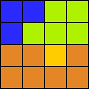
Original Image. |
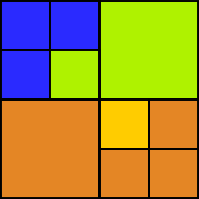
Quadtree representation of the image. |
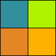
Quadtree representation with a higher tolerance value |
 |
Example on Photograph
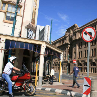 Original image. Original image. |
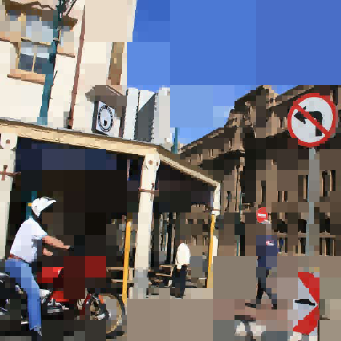 Quadtree compressed image. Quadtree compressed image. |
To implement a quad tree, you need to do five things:
- define a QuadTree class;
- define a Node class;
- implement a detail measuring function;
- implement a construction algorithm;
- implement an access algorithm.
These are explained below.
Defining the Quad Tree Class
This class is very simple: it stores the root node and the algorithms, which are explained in the sections below. Here is how that would look in Java:
class Quadtree
{
  Node root;

  QuadTree(Grid grid)
  {...}

  Color get(int x, int y)
  {...}
}
Defining the Node class
The node class is where most of the work is done. It should store its four children (possibly all Null), and be able to handle construction and access functions.
class Node
{
  Node children[];
  int x, y;
  int width, height;

  Node(Grid grid, int x, int y, int width, int height)
  {...}

  Color get(int x, int y)
  {...}
}
Detail Measure Algorithm
This algorithm calculates the amount of detail on a rectangle of the grid. How that detail is measured, depends on the application. For images, the average Manhattan distance between colours and the average colour is a crude measure that often works well. The Manhattan distance between two colours is defined as:
d = |r1 – r2| + |g1 – g2| + |b1 – b2|,
Where ‘r1’ is the red component of colour 1, and so on. Note that the entire grid is passed to the algorithm, with extra parameters to indicate the boundaries of the piece we actually want to measure. We also define a help function to calculate the average of a rectangle in a grid.
// Calculates the average color of a rectangular region of a grid
Color average(Grid grid, int x, int y, int width, int height)
{
  int redSum = 0;
  int greenSum = 0;
  int blueSum = 0;

  //Adds the color values for each channel.
  for(int i = 0; i < x + width; i++)
  {
    for(int j = 0; j < y + height; j++)
    {
      Color color = grid.get(i, j);
      redSum += color.getRed();
      greenSum += color.getGreen();
      blueSum += color.getBlue();
    }
  }

  //number of pixels evaluated
  int area = width * height;

  // Returns the color that represent the average.
  return Color(redSum / area, greenSum / area, blueSum / area);
}

// Measures the amount of detail of a rectangular region of a grid
Color measureDetail(Grid grid, int x int y, int width, int height)
{
  Color averageColor = average(grid, x, y, width, height);
  int red = averageColor.getRed();
  int green = averageColor.getGreen();
  int blue = averageColor.getBlue();
  int colorSum = 0;

  // Calculates the distance between every pixel in the region
  // and the average color. The Manhattan distance is used, and
  // all the distances are added.
  for(int i = 0; i < x + width; i++)
  {
    for(int j = 0; j < y + height; j++)
    {
      Color cellColor = grid.get(i, j);
      colorSum += abs (red – cellColor.getRed());
      colorSum += abs(green – cellColor.getGreen());
      colorSum += abs (blue – cellColor.getBlue());
    }
  }

  // Calculates the average distance, and returns the result.
  // We divide by three, because we are averaging over 3 channels.
  return colorSum / (3 * area);
}
Construction Algorithm
The construction algorithm can be put in the constructor of the Node class. The constructor of the actual QuadTree class simply constructs the root node. The algorithm is simple: the detail is measured over the part of the grid that the node is meant to represent. If it is higher than some threshold, the node constructs four children nodes, each representing a quadrant of the original rectangle. If the detail in the rectangle is lower than the threshold, the average colour is calculated for the rectangle, and stored in the node.
The threshold value passed to the function is often determined empirically – that is, you change it until you get what you want. Obviously, the smaller it is, the more accurately the quadtree will represent the original data, and the more memory and processing time will be used.
// Constructs a new Quadtree node from a grid, and parameters
// that indicate the region this node is to represent, as well as
// the threshold to use to decide wether to split this node further.
Node(Grid grid, int x, int y, int width, int height, float threshold)
{
  this.x = x;
  this.y = y;
  this.width = width;
  this.height = height;

  if (measureDetail(grid, x, y, width, height) < threshold)
  {//too little detail
    color = average(grid, x, y, width, height);
  }
  else
  {
    //enough detail to split
    children = new Node[4];

    //upper left quadrant
    children[0] = new Node(data, x, y, width/2, height/2);

    //upper right quadrant
    children[1] = new Node(data, x + width/2, y, width - width/2, height/2);

    //lower left quadrant
    children[2] = new Node(data, x, y + height/2, width/2, height - height/2);

    //lower right corner
    children[3] = new Node(data, x + width/2, y + height / 2,

    width - width/2, height - height/2);
  }
}
Access Algorithm
The access works as follows: if the node from which the method is called is a leaf (a node without any children), that node’s colour is returned. Otherwise, the call is delegated to the child node of the correct quadrant. The method is shown below:
// Returns whether this node has any children.
boolean isLeaf()
{
  return children == null;
}

 // Gets the colour at the given pixel location.
Color get(int i, int j)
{
  if isLeaf()
  {
    return color;
  }
  else
  { // Decides in which quadrant the pixel lies,
    // and delegates the method to the appropriate node.

    if(i < x + width/ 2)
    {
      if(j < y + height / 2)
      {
        return ((Node) children[0]).get(i, j);
      }
      else
      {
        return ((Node) children[2]).get(i, j);
      }
    }
    else
    {
      if(j < y + height / 2)
      {
        return ((Node) children[1]).get(i, j);
      }
      else
      {
        return ((Node) children[3]).get(i, j);
      }
    }
  }
}
Real-world Implementation
The typical real-world implementation will differ in several respects from the simple implementation described above:
- Integers will be used to represent colours in the raw data and Nodes, rather than Colour objects.
- Intermediate values of colours will be stored as floats, where component values are scaled to lie between 0 and 1; Whatever detail function is used, its output will be scaled to lie between 0 and 1. (This makes it easier to determine a correct threshold).
- Adding several hundred (or even thousand) red, blue and green values will cause overflow problems.
- The summands are often scaled before they are added (for example, the division by the area can be done before they are added to the sums).
- Calculating the average is expensive; where it is used as part of the detail measuring algorithm, it will be calculated separately, and passed to this function, so that the value can be reused.
Debugging Tips
- Implement a way to visualize the quad tree, even if the quad tree does not represent an image. In addition to the normal visualization, also implement visualizations that
- render every square in a different colour (see example algorithms http://arxiv.org/abs/cs.CG/9907030); render outlines of blocks over the normal visualization.
- Implement a visualization of the error of your quad tree representation against the original.
- For benchmarking, implement node count methods for counting
- all nodes;
- all leaf nodes.
- This is useful to make sure that a quad tree is indeed a more efficient representation of you data (for example, white noise will be better represented by a grid).
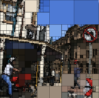
Quadtree image with grid visualization.
Resources
http://www.ics.uci.edu/~eppstein/gina/quadtree.html A list of quadtree resources from Geometry in Action.
Downloads
You can download examples of implementations in Python on code-spot:
Pingback: code-spot · Quadtrees
You did not specify the type of threshold, and you got “this.y = x” in the construction of a node. Just thought I’s point it out 😉
Thank you! I fixed it.
You mentioned ” In part 2 we will look at more general applications, such as occupancy
maps and force fields. We also look at the properties of data that
determines whether it is suitable to represent as a quadtree.” Is there a part 2? If so can you add the link?
Thanks,
MJ
It’s actually in one of the old PDF mags: http://devmag.org.za/uploads/DevMag_Issue27.zip
now the link is not available. can u mail me
remyaksasi@gmail.com